
The Lithos Manifesto: Anatomy of a Storage Engine
“Why build a database from scratch in C? Aren’t there libraries for that?”
Yes. There are libraries.
But I didn’t want a library. I wanted to know how bytes actually hit the disk.
NOTE: This blog is written for engineers who want to understand databases from first principles, not for application developers looking for abstractions. This will take a while to read, but it will be worth every minute.
Prologue: The Abstraction Trap
Most software engineers live their entire lives inside a simulation.
You write const user = await db.user.create({ name: "Aditya" });.
The command goes into the ether. It travels through an ORM, then a database driver, then a TCP socket, then a kernel buffer, then a filesystem driver, then a disk controller, and finally, miraculously, a few magnetic grains flip on a platter, or a few electrons get trapped in a floating gate transistor.
It just works. Until it doesn't.
Until you hit 10,000 writes per second and your latency spikes to 5 seconds.
Until your server crashes and you lose the last 5 minutes of data because you didn't understand fsync.
Until you run out of RAM because you didn't know how your database handles compaction.
To the average dev, the database is a "Black Box". It is magic.
And "magic" is dangerous.
I was tired of the magic.
I wanted to break the box open. I wanted to see what's inside.
How it works. Why it works the way it does.
So, I did the only logical thing a sane person would do in the big 2025:
I wrote a production-grade storage engine from scratch in C.
No Rust. No Go. No Garbage Collector. No Runtime.
Absolutely none of that.
Just libc, pthreads, and the cold, hard reality of the Linux Kernel.
This is the story of Lithos.
And more importantly, this is a manual on how to build your own database.
So sit back, and buckle up, because this is gonna be a long, and fun read :)
PART I: THE PHYSICS OF DATA
Chapter 1: The Layer Cake of Lies
Before we write a single line of code (struct Lithos_DB), we need to understand where we are coding.
When you use a high-level language, the computer lies to you.
- Java/Go: "Here you go my sweetheart. Here is infinite memory. Just
new Object()"- The Lie: Memory is NOT infinite. Allocation is expensive (
malloctakes CPU cycles). Garbage Collection pauses EVERYTHING to clean up your mess.
- The Lie: Memory is NOT infinite. Allocation is expensive (
- Python/JS: "Here is a List. Append to it for as long as you want :)"
- The Lie: That list is a dynamic array. When it fills up, the language pauses, allocates a new double-sized array, copies every single element over, and deletes the old one.
Guess what? You just spiked your CPU usage and didn't know why.
- The Lie: That list is a dynamic array. When it fills up, the language pauses, allocates a new double-sized array, copies every single element over, and deletes the old one.
But in C, the lies stop.
In C, you are standing naked in front of the machine.
If I want to store a Key-Value pair, I have to ask:
- How many bytes is it?
- Where do those bytes live? (Stack? Heap? mmap?)
- How long do they live? (Do I free them now? Later? Never?)
- How does the CPU see them? (Are they aligned to 8 bytes? Will they cause a cache miss?)
Lithos is built on the philosophy of Absolute Control.
We do not ask the OS for memory one byte at a time. We grab 4MB chunks and manage them ourselves.
We do not let the OS decide when to write to disk. We force it with fsync.
If you want to build high-performance systems, you have to stop trusting the abstractions and become the manager yourself.
Chapter 2: The Physics of Spinning Rust (And Why B-Trees Fail)
To design a database, you must first choose a Data Structure.
And to choose a Data Structure, you must understand the hardware it runs on.
Your Hard Drive (or SSD) has a physical personality.
The Myth of Random Access
We call it "RAM" (Random Access Memory) because jumping to byte 0 takes the same time as jumping to byte 1,000,000.
Disks are NOT Random Access.
Imagine a Hard Drive is a literal Record Player.
To read a song, the needle has to physically move to the right groove.
- Seek Time: The time it takes the needle to move. (~5-10ms).
- Read Time: The time it takes to actually play the music. (Nanoseconds).
If you ask the disk to read 100 random files, it spends 99% of its time moving the needle and 1% of its time reading data.
This is Random I/O. It is slow. It is the enemy.
The B-Tree Problem
Most traditional databases (Postgres, MySQL, Oracle) use B-Trees.
A B-Tree keeps data sorted on disk at all times.
If you have a file with users [Aman, Krishna] and you want to insert Baldev:
- The DB finds the exact spot on the disk between Aman and Krishna.
- It reads that page into RAM.
- It rewrites the page:
[Aman, Baldev, Krishna]. - It writes it back to the exact same spot on the disk.
If you insert 10,000 random users, the disk needle is jumping around like crazy.
Your write throughput COLLAPSES.
The Solution: The Log-Structured Merge Tree (LSM)
Used by LevelDB, RocksDB, BigTable, and most importantly, Lithos.
The philosophy of LSM is simple:
Never modify existing data.
Only append new data.
If you want to insert Baldev:
- You don't find the old page.
- You just write
Baldevto the very end of the file.
If you want to update Aman's name:
- You don't overwrite the old
Amanrecord. - You write a new record at the end:
Aman = NewName.
Because we are always appending to the end, the disk needle never has to jump back. It just writes in a straight line.
This converts Random Writes into Sequential Writes.
Sequential Writes are 100x faster than Random Writes.
And fun fact: this is why Lithos can handle 73,000 writes per second on my laptop, while SQLite dies out at 2,000.
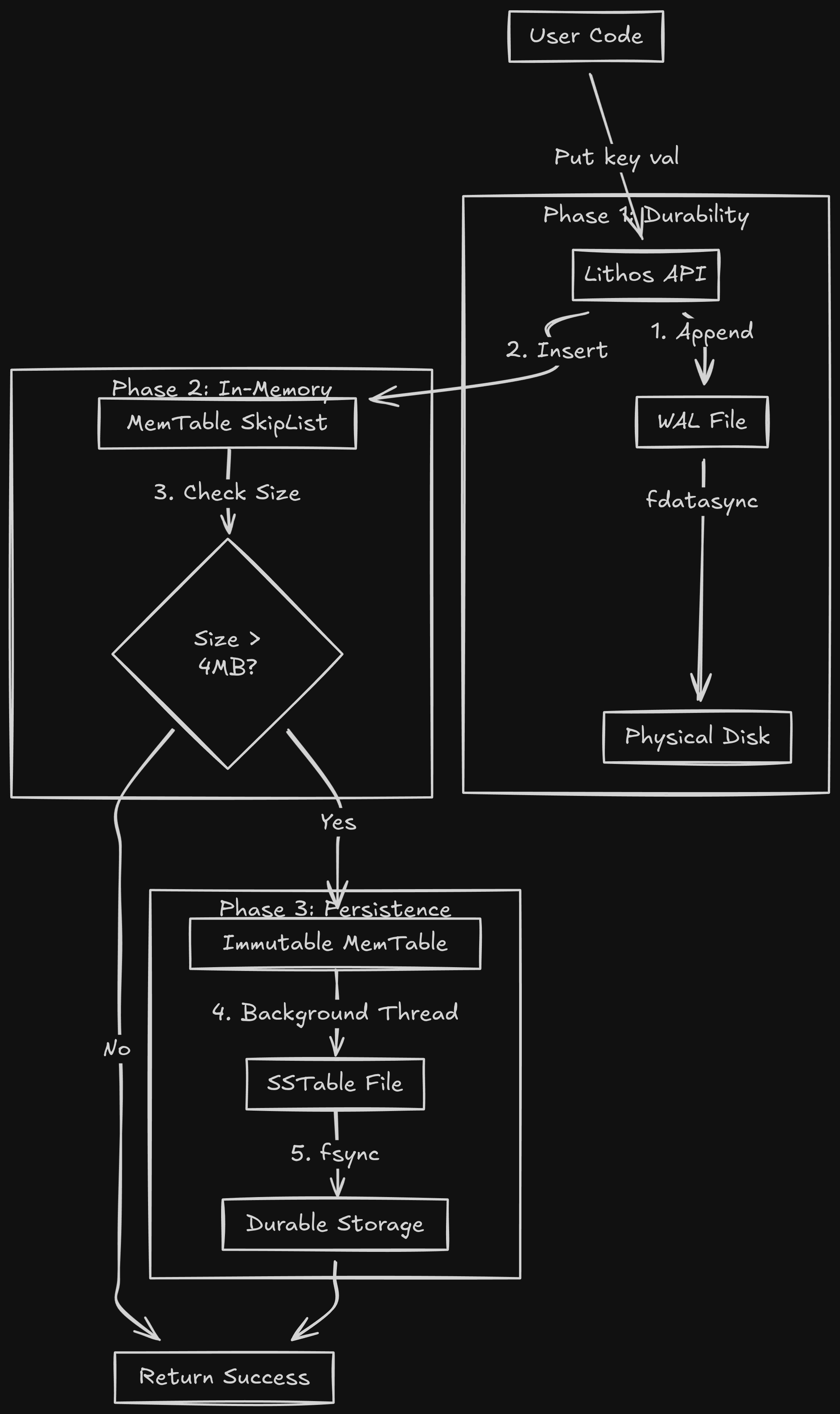
Chapter 3: The Architecture of Lithos
So, we chose the LSM-Tree. Now, how do we build it?
We need a pipeline that moves data from Volatile Memory to Persistent Storage.
We break the engine into three layers.
Layer 1: The Volatile Memory (RAM)
- Component:
MemTable - Data Structure: SkipList
- Speed: Nanoseconds.
When a write comes in, it goes here first.
But RAM is volatile. If I pull the power plug, this data vanishes.
We cannot lose data. So we need a safety net.
Layer 2: The Safety Net (WAL)
- Component:
LogWriter - File:
wal.log - Speed: Microseconds.
Before we touch the MemTable, we append the operation to a simple log file on disk.
PUT key=user:1 val=aditya -> Append to file -> fsync().
If the server crashes, we can replay this log to rebuild the RAM.
Layer 3: The Persistent Storage (Disk)
- Component:
SSTable(Sorted String Table) - File:
*.sst - Speed: Milliseconds.
Eventually, RAM fills up (default: 4MB). We can't keep data there forever.
When the MemTable is full, we:
- Freeze it (make it Immutable).
- Sort it.
- Flush it to a file on disk.
This file is an SSTable. It is Immutable. Once written, Lithos NEVER opens it for writing again.
This solves nearly all concurrency bugs. If a file never changes, you don't need locks to read it.
The Full Lifecycle Diagram
Chapter 4: The Toolchain (Or: Why I Used Make)
Before we start coding, we need a build system.
Modern C++ uses CMake. It is powerful. It is also bloated as hell.
For Lithos, I used GNU Make.
Why?
Because Make is honest.
A Makefile is just a list of shell commands.
- "To build
lithos.o, takelithos.cand rungcc -c lithos.c." - "To build the binary, take all
.ofiles and link them."
There is no magic. There is no hidden dependency graph.
If the build fails, I know exactly which command failed.
The Compiler Flags:
We compile with -std=c11.
And we use the Holy Trinity of Sanitizers (enabled with make SANITIZE=1):
ifeq ($(SANITIZE),1)
CFLAGS += -fsanitize=address -fsanitize=undefined -fno-omit-frame-pointer
LDFLAGS += -fsanitize=address -fsanitize=undefined
endif
- AddressSanitizer (ASan): Detects memory leaks, buffer overflows, and use-after-free bugs instantly.
- UndefinedBehaviorSanitizer (UBSan): Detects integer overflows, null pointer dereferences, and other C sins.
Building a database in C without Sanitizers is like driving a car blindfolded. You might make it, but it's highly likely you'll crash and burn.
PART II: THE HOT PATH (WRITES)
Now, we are going to build the "Hot Path"; the code that runs every single time a user sends a PUT request.
This involves three critical components working in harmony:
- The WAL: Ensuring data survives a power outage.
- The Arena: Managing memory without
mallocoverhead. - The SkipList: Organizing data in RAM without locking the world.
Time to get coding.
Chapter 5: The Lifeline (Implementing the WAL)
When a write comes in, the very first thing we do is secure it.
We append it to a log file (wal.log) and flush it to disk.
The Problem with write()
You might think writing to a file is easy:
write(fd, "key=value", 9);
Wrong.
When you call write() in Linux, the data doesn't go to the disk. It goes to the Page Cache (RAM). The OS decides when to flush that cache to the physical platter. It might be 5 seconds later.
If the power cuts in those 5 seconds, you lied to the user. You said "Success", but the data is gone.
The Fix: fdatasync()
We must force the OS to flush.
write(fd, data, len);
fdatasync(fd); // BLOCK until electrons hit the magnetic platter
This is slow. True.
But it is honest.
And just like we were all taught in our childhoods, "honesty is the best policy."
The Binary Format
We don't just dump raw text into the file. If we crash while writing, we might end up with half a message. We need a structure that allows us to detect corruption.
I chose a Block-Based Log Format (inspired by LevelDB).
The log is a sequence of 32KB Blocks.
Why 32KB to be precise?
- Alignment: 32KB is a multiple of the standard 4KB OS Page size.
- CPU Efficiency: It keeps the CPU pipeline fed. Processing 1 byte at a time is cache-suicide.
The Record Header:
Every entry in the log has a 7-byte header:
// Header layout (7 bytes total):
// [0-3]: CRC32 checksum (4 bytes)
// [4-5]: Length of payload (2 bytes, little-endian)
// [6]:   Record type (1 byte)

#define kHeaderSize 7

// The header is written as raw bytes:
char header[kHeaderSize];
EncodeFixed32(header, crc);      // Bytes 0-3
header[4] = (length & 0xff);      // Byte 4
header[5] = (length >> 8) & 0xff; // Byte 5
header[6] = (char)type;           // Byte 6
Handling Massive Records (Fragmentation)
What if a user wants to store a 100KB JSON blob? It won't fit in a 32KB block.
We can't resize the block (that breaks alignment).
Well, in that case, we have to slice the data.
Note: A single record fragment can be at most 65535 bytes (kMaxRecordSize), which is the max value of a 2-byte length field.
We use the type field to track this:
kFullType (1): The record fits entirely in this block.kFirstType (2): This is the first chunk of a massive record.kMiddleType (3): This is a middle chunk.kLastType (4): This is the final chunk.
The Recovery Logic:
When Lithos restarts after a crash, it reads the log file from top to bottom.
It acts like a state machine.
- Read a record.
- Calculate the CRC32 of the payload. Does it match the header?
- No? CORRUPTION DETECTED. Stop reading immediately. Truncate the log here.
- Yes? Continue.
- Check the type.
- If
kFirstType, start a buffer. - If
kMiddleType, append to buffer. - If
kLastType, finish buffer and insert into DB.
This guarantees Atomicity. We never insert half a record.
Chapter 6: The Arena (Memory Management)
Now that the data is safe on disk, we need to put it into RAM so we can read it.
We need to allocate a node for our SkipList.
Why malloc is the Enemy
In a high-throughput database, you might do 50,000 writes per second.
Calling malloc(64) 50,000 times a second is shooting yourself in the head.
Why, you ask?
- Syscall Overhead:
mallocmight need to ask the kernel for more RAM (sbrkormmap). This involves a context switch. - Fragmentation: Allocating millions of tiny 64-byte objects creates "holes" in the heap that are hard to reuse.
- Cache Locality:
mallocmakes no guarantees about where the memory is. Node A might be at address0x1000and Node B at0x9000. The CPU pre-fetcher hates this.
So, what's the fix for this?
The Solution: The Arena Allocator
An Arena is the simplest memory allocator possible.
It is a "Bump Pointer" allocator.
How it works:
- We ask the OS for a big chunk (e.g., 4KB or 4MB).
- We keep a pointer
alloc_ptrto the start. - When you want
Nbytes, we simply returnalloc_ptrand increment it byN.
// internal representation
struct Arena {
    char* alloc_ptr;           // Current free position
    size_t alloc_bytes_remaining; // Bytes remaining in current block

    char** blocks;             // Dynamic array of all big blocks we own
    size_t blocks_count;       // Number of blocks allocated
    size_t blocks_capacity;    // Capacity of blocks array

    _Atomic size_t memory_usage; // Total memory used (atomic for thread-safety)
};

char* Arena_Allocate(Arena* a, size_t bytes) {
    // 1. Alignment (Crucial)
    // Pointers on 64-bit CPUs should be 8-byte aligned.
    // If we return address 0x1001, the CPU has to do two fetches to read a uint64.
    // So we pad the request.
    const size_t kAlignment = 8;
    size_t aligned_bytes = (bytes + kAlignment - 1) & ~(kAlignment - 1);

    // 2. Check space
    if (a->alloc_bytes_remaining < aligned_bytes) {
        // Fallback: Allocate a new 4KB block from the OS
        char* new_block = AllocateNewBlock(4096);
        AddBlock(a, new_block); // Add to our blocks array
        a->alloc_ptr = new_block;
        a->alloc_bytes_remaining = 4096;
    }

    // 3. Bump & Return
    char* result = a->alloc_ptr;
    a->alloc_ptr += aligned_bytes;
    a->alloc_bytes_remaining -= aligned_bytes;
    return result;
}
The "Free" Magic:
We don't implement Arena_Free(ptr).
We don't need to free individual keys.
The MemTable is immutable. Once data is in there, it stays there until the whole table is flushed to disk.
When we flush, we free the entire Arena at once.
Millions of keys. One free() per block.
This is efficient. This is fast.
Just perfect.
Memory Tracking:
The Arena maintains an atomic counter (_Atomic size_t memory_usage) to track total memory usage across all blocks. This allows the database to know when the MemTable has reached its size limit (4MB) without expensive calculations.
Large Allocation Strategy:
If you request a very large allocation (> 1KB), the Arena allocates a dedicated block for just that allocation, instead of wasting the rest of the current block. This prevents fragmentation when storing large values.
Chapter 7: The SkipList (The Core Data Structure)
We have the memory. Now we need to organize it.
We need a data structure that keeps keys sorted (A, B, C...) so we can scan them.
Why not a Binary Search Tree?
Standard databases use Red-Black Trees or AVL Trees.
These are great, but they require Rebalancing.
If I insert 1, 2, 3, 4, 5 into a standard BST, it becomes a straight line (Linked List). Performance drops to O(N).
To fix this, the tree has to "rotate" nodes.
Rotation is a write operation. It touches multiple nodes.
To do this safely in a multi-threaded environment, you have to Lock the nodes.
If you lock the root, nobody else can read or write.
Enter The SkipList
A SkipList is a Probabilistic Data Structure.
It replaces "strict rotation rules" with "coin flips."
Imagine a Linked List where every node is a tower.
- All towers have a Level 0 link (next node).
- Some towers have a Level 1 link (skips 1 node).
- Few towers have a Level 2 link (skips 5 nodes).
Searching:
You start at the highest level (the express lane).
You jump forward until you overshoot your target.
Then you drop down a level and continue.
This gives O(log N) search performance, just like a Tree.
Insertion (The Magic):
When we insert a new key, we roll a dice to decide how tall its tower is.
Lithos uses a branching factor of 4 (not 2), with a max height of 12:
- 75% chance: Height 1
- ~19% chance: Height 2
- ~5% chance: Height 3
- Maximum height: 12 levels
Here's the actual algorithm:
static int RandomHeight(unsigned int *seed) {
    int height = 1;
    while (height < SKIPLIST_MAX_HEIGHT &&
           (Random_Next(seed) % SKIPLIST_BRANCHING == 0)) {
        height++;
    }
    return height;
}
Each time through the loop, there's a 1-in-4 (25%) chance of continuing.
Why this is better for Concurrency:
Because the height is random, we don't need to rotate the tree.
Inserting a node only affects its immediate neighbors.
We can implement this using Atomic Operations (Compare-And-Swap).
This means:
- Writers only lock a small part of the list.
- Readers don't lock at all. They can walk the list while it's being modified.
The C Implementation Details
This was the hardest part of Lithos to get right.
The actual constants used in Lithos:
#define SKIPLIST_MAX_HEIGHT 12
#define SKIPLIST_BRANCHING 4  // 1 in 4 chance of increasing height
1. The Node Structure:
We use a "Flexible Array Member" for the next pointers, because different nodes have different heights.
typedef struct SkipList_Node {
    const void* key;  // Points to the encoded memtable entry
    // Flexible array member: size determined at allocation
    // Each level has an atomic pointer to the next node
    _Atomic(uintptr_t) next[];
} Node;
The key insight: we store uintptr_t (integer addresses) instead of direct pointers, then cast them. This gives us finer control over atomic operations and memory ordering.
2. Memory Ordering is a Nightmare
When linking a new node, the order of operations matters.
If you update the "Previous Node" to point to "New Node" before you initialize "New Node", a reader might jump to "New Node" and see garbage.
We need Memory Barriers.
// Correct Order:
// 1. Set NewNode->Next = OldNext
atomic_store_explicit(&new_node->next[i], old_next, memory_order_relaxed);

// 2. Barrier. Ensure step 1 is visible to all CPUs before step 3.
atomic_thread_fence(memory_order_release);

// 3. Set PrevNode->Next = NewNode
atomic_store_explicit(&prev_node->next[i], new_node, memory_order_release);
If you get this wrong (and oh boy did I, multiple times), you get elusive bugs that only happen once every 10 hours on a 16-core server.
Chapter 8: Putting it Together (The Put Path)
So, here is the full code path for Lithos_Put:
- Lock the DB:
pthread_mutex_lock(&db->mutex).
- Wait, a lock?
Yes, Lithos allows only One Writer at a time. This simplifies the WAL append logic. The SkipList allows concurrent reads, but writes are serialized.
- Write to WAL:
- Calculate CRC32.
- Fragment if needed.
write()+fdatasync().
- Write to MemTable:
- Allocate node from Arena.
- Encode the entry: The MemTable stores entries in a specific format:
[InternalKeySize varint][UserKey][Seq+Type 8 bytes][ValueSize varint][Value] - Insert into SkipList (dealing with atomic pointers).
- Check Size:
- Has the MemTable grown > 4MB?
- If yes, trigger a Switch.
imm = mem(Current memtable becomes immutable).mem = new MemTable.- Signal the background thread: "Hey, flush
immto disk."
- Unlock:
pthread_mutex_unlock(&db->mutex).
This whole process takes about 13 microseconds on my laptop.
That is 73,000 writes per second.
Note on Performance: These numbers are from sequential writes with fdatasync() enabled. The throughput is primarily limited by:
- The cost of
fdatasync()(forcing data to physical storage) - The mutex serializing writes
- Disk I/O characteristics
With sync=false (disabling fdatasync), throughput can exceed 500,000 writes/sec, but at the cost of durability.
But eventually, RAM fills up. We have to flush to disk.
And that brings us to the most complex part of the engine: The SSTables.
PART III: THE COLD PATH (DISK)
"RAM is a suggestion. Disk is a commitment."
We need to move data from the "Hot" tier (RAM) to the "Cold" tier (Disk).
We need to turn our dynamic, mutable SkipList into a static, immutable file.
Welcome to the world of SSTables.
Chapter 9: The Freeze (Moving from RAM to Disk)
The transition from RAM to disk must be seamless. We cannot stop accepting writes while we flush 4MB of data to a slow HDD. That would cause massive latency spikes.
We solve this with a Double Buffering technique.
The Trigger
Every time a write finishes, we check the size of the active MemTable (mem).
if (mem->approximate_memory_usage > options.write_buffer_size) {
    // It's too big. Trigger a flush.
}
By default, this limit is 4MB. The "approximate" memory usage is tracked by the Arena's atomic counter, which includes all allocations (keys, values, skiplist nodes, and internal overhead).
The Swap (The Critical Section)
This is the only part of the write path that requires a global lock on the database.
- Acquire Lock:
pthread_mutex_lock(&db->mutex). - Wait for Background Worker: If the background thread is already busy flushing a previous table, we must wait. (We use a
pthread_cond_tcondition variable here). - The Switch:
- We take the current active pointer
memand move it toimm(Immutable MemTable). - We create a brand new, empty
MemTableand assign it tomem. - We create a new Write-Ahead Log file for the new
mem.
- Signal Background Worker: "Hey,
immis ready to be flushed." - Release Lock:
pthread_mutex_unlock(&db->mutex).
This whole process takes microseconds. The main write path is unblocked almost instantly.
The Background Flush
Meanwhile, in a separate thread, the background worker wakes up.
It sees the imm pointer has data.
It takes that entire SkipList, sorts it, and starts streaming it into a file.
Once the file is successfully written to disk (fsync'd):
- It deletes the old Write-Ahead Log corresponding to that data (we don't need it anymore, the data is safe on disk).
- It destroys the
immMemTable (freeing the Arena).
Chapter 10: The Anatomy of an SSTable
So, what does this file look like?
We call it an SSTable (Sorted String Table).
A naive approach would be to just write KeyLen|Key|ValLen|Value over and over again in a flat file.
Speaking from experience, this is a TERRIBLE idea.
If you have a 1GB file, and you want to find key "zebra", you would have to read the entire 1GB file from start to finish to find it.
That's slow.
We don't like slow.
So, we need structure. We need an index.
The Block-Based Format
Lithos organizes the SSTable into Blocks.
Just like the WAL, these are usually 4KB to align with OS pages.
+-----------------------------+
| Data Block 0 (Keys A-F)     | <-- 4KB compressed
+-----------------------------+
| Data Block 1 (Keys G-M)     | <-- 4KB compressed
+-----------------------------+
| ...                         |
+-----------------------------+
| Filter Block (Bloom Filter) | <-- Fast lookup hack
+-----------------------------+
| Index Block                 | <-- The map to find data blocks
+-----------------------------+
| Footer                      | <-- Fixed size, points to Index
+-----------------------------+
1. The Data Blocks
These hold the actual key-value pairs. They are sorted.
2. The Index Block
This is the map. It tells us which range of keys lives in which Data Block.
It stores the largest key in each block and the offset of that block.
Example Index:
- Key "F": Block 0 starts at offset 0.
- Key "M": Block 1 starts at offset 4096.
- Key "Z": Block 2 starts at offset 8192.
When we want to find "banana":
- We load the Index Block.
- We binary search the index. "banana" is less than "F".
- Therefore, if "banana" exists, it MUST be in Block 0.
- We only perform one disk seek to read Block 0.
3. The Footer
How do we find the Index Block? It's at the end of the file, but the file size varies.
The Footer is a Fixed Size block (48 bytes) at the very absolute end of the file. It contains a "Magic Number" to verify it's a valid Lithos table, and pointers (offsets) to the Index and Filter blocks.
To open an SSTable, you read the last 48 bytes first.
Chapter 11: Squeezing Bits (Prefix Compression)
If we just store raw keys, we waste enormous amounts of space.
Database keys are rarely random. They look like this:
user:100:name
user:100:email
user:101:name
user:101:email
They share massive prefixes. Storing user: four times is, well, wasteful.
The Prefix Compression Algorithm
Lithos uses incremental prefix compression within Data Blocks.
When writing a key, we compare it to the previous key we just wrote.
- Key 1:
user:100:name
- Shared: 0
- Unique: 13 (
user:100:name) - Store full key.
- Key 2:
user:100:email
- Compare to prev: They share
user:100:(9 bytes). - Shared: 9
- Unique: 5 (
email) - Store only
9andemail.
On disk, it looks like this (using Varints for lengths):
[SharedLen] [UniqueLen] [ValLen] [UniqueKeyBytes] [ValueBytes]
This shrinks typical datasets by 30-50%.
The Problem: Random Access
Compression introduces a massive problem.
If I want to read Key 50 in a block, I can't just jump to it. It's compressed relative to Key 49, which is compressed relative to Key 48...
I have to decode everything from Key 1 sequentially. That's too slow for a read query.
The Solution: Restart Points
We need to compromise between compression density and read speed.
So we introduce Restart Points.
Every N keys (controlled by block_restart_interval option, typically 16), we force the compression to reset.
We write the full, uncompressed key. We record the offset of this key in a "Restart Array" at the end of the block.
When we search inside a block:
- We binary search the Restart Array to find the closest restart point before our target key.
- We jump to that offset. We know this key is fully readable.
- We start linearly scanning and decoding from there until we find our key.
This ensures we never have to linearly scan more than 16 keys, keeping reads fast while still getting good compression.
Chapter 12: The Speed Hack (Bloom Filters)
Even with the Index Block, reading from disk is slow.
Imagine you have 5 levels of LSM trees, totaling 100 SST files.
To find a key, you might have to check the Index Block of all 100 files. That's 100 potential disk seeks.
If the key doesn't exist, you just wasted huge amounts of I/O resources to confirm a negative.
We need a way to quickly know if a file might contain a key, without actually reading the data blocks.
The Nightclub Bouncer Analogy (Thanks Gemini)
Think of an SSTable as a nightclub. The Data Blocks are the people inside.
Checking the Index Block is like opening the door and yelling out a name to see if they respond. It takes effort.
A Bloom Filter is the Bouncer at the door with a clipboard.
You ask the bouncer: "Is 'Aditya' inside?"
The Bloom Filter can give two answers:
- "Definitely Not." (Go away. Don't open the door.)
- "Maybe." (He might be. You have to go inside and check.)
It will never give a false negative. If it says "No", the key is 100% guaranteed not to be there.
It might give a false positive (say "Maybe" when the key isn't there).
But thankfully, we tune the math to keep this rate low (~1%).
How it Works (The Math)
A Bloom Filter is just a bit array (a long string of zeros: 000000...).
When we create the SSTable, we take every key and run it through several hash functions.
Let's say we have an array of 10 bits and we use the same hash function with different seeds (delta).
Lithos uses k hash functions where k is calculated based on bits_per_key (default 10).
For 10 bits per key, we use approximately k=7 hash functions (calculated as 0.69 * bits_per_key).
Insert "Key A":
Hash1("Key A") % 10 = 2-> Set bit 2 to1.Hash2("Key A") % 10 = 7-> Set bit 7 to1.
Array:0010000100
Insert "Key B":
Hash1("Key B") % 10 = 4-> Set bit 4 to1.Hash2("Key B") % 10 = 7-> Set bit 7 to1. (Already set, that's fine).
Array:0010100100
Now, we query:
Check for "Key C":
Hash1("Key C") % 10 = 1. Is bit 1 set? No.- Result: Definitely Not. Stop. Do not read disk.
Check for "Key A":
Hash1("Key A") % 10 = 2. Is bit 2 set? Yes.Hash2("Key A") % 10 = 7. Is bit 7 set? Yes.- Result: Maybe. (All hashes matched bits that were set to 1). Now we must pay the cost to read the Index Block and confirm.
The Impact
Bloom Filters are stored in their own block in the SSTable. They are small enough to usually stay cached in RAM.
For a workload that requests lots of non-existent keys, Bloom Filters reduce disk I/O by 99%. It is the single best optimization in the entire database engine.
PART IV: THE READ PATH (TIME)
"Writing is O(1). Reading is O(WTF)."
When a user asks Get("user:100"), where is it?
- Is it in the active MemTable?
- Is it in the Immutable MemTable waiting to flush?
- Is it in the Level-0 SSTable on disk?
- Is it in the Level-1 SSTable from last week?
Even worse: It might be in ALL of them.
Maybe you wrote user:100 = "Aman" last week (Level 1), and updated user:100 = "Baldev" today (MemTable).
The database must return "Baldev".
We need a system to unify these scattered fragments into a single, coherent truth.
Chapter 13: The Hierarchy of Freshness
The first rule of reading in an LSM tree is simple: Freshness Wins.
We search components in reverse chronological order. The first match we find is the correct one.
The search hierarchy looks like this:
- Active MemTable: (Most Recent). Fast RAM lookup (
O(log N)SkipList). - Immutable MemTable: (Recent). Fast RAM lookup.
- Level 0 Files: (Newest Disk Data). These are just flushed MemTables. Note: Level 0 files can overlap. We might have to check all of them.
- Level 1 Files: (Older). Sorted and non-overlapping. We binary search to find exactly one file.
- Level 2+: (Ancient). Same as Level 1.
The moment we find the key, we stop.
This implies that reading recent data is very fast (it's in RAM).
Reading old data is slower (it's deep in Level 4).
Chapter 14: The Iterator Abstraction
We have data in SkipLists (RAM pointers) and SSTables (Disk offsets).
We can't write different code for each. We need a common interface.
Enter the Iterator.
In C (simulating an interface using function pointers, similar to a vtable), it looks like this:
typedef struct Lithos_Iterator {
    void* state;
    void (*Seek)(void* state, Slice target);
    void (*SeekToFirst)(void* state);
    void (*Next)(void* state);
    bool (*Valid)(void* state);
    Slice (*Key)(void* state);
    Slice (*Value)(void* state);
    // ... cleanup ...
} Lithos_Iterator;
We implement this interface for everything:
MemTableIterator: Wraps the SkipList.BlockIterator: Iterates inside a 4KB disk block.TwoLevelIterator: Uses the Index Block to jump between Data Blocks in an SST file.
Now, whether data is in RAM or on Disk, we treat it exactly the same: Iter->Seek(), Iter->Next().
Chapter 15: The Merging Iterator (The Tournament)
This is genuinely one of the coolest algorithms in database engineering.
Imagine you want to run a Scan() (iterate over all keys).
You have:
- Iterator A (MemTable):
[apple, dog, zebra] - Iterator B (Disk):
[banana, cat, elephant]
You want the combined output: [apple, banana, cat, dog, elephant, zebra].
We build a MergingIterator.
It holds an array of child iterators (A and B).
It maintains a Min-Heap (Priority Queue).
How it works:
- Initialize A and B. Push them into the Heap.
- The Heap top is the iterator with the smallest current key.
- Top is A (
apple).
- Output
apple. - Advance A. A is now
dog. - Fix the Heap.
- Heap has: B (
banana), A (dog). - New Top is B.
- Output
banana. - Advance B. B is now
cat. - Fix Heap...
This allows us to merge N sorted streams into one sorted stream efficiently.
When you call Lithos_Scan, you are actually driving a MergingIterator that is driving a MemTableIterator and 100 SSTableIterators in a synchronized dance.
Chapter 16: Time Travel (MVCC)
Now for the hard part. Concurrency.
In a naive database, if I am reading Key A, and you write Key A, we need a lock. I wait. You write. I read.
This is slow.
And like I said earlier, we do NOT like slow.
So, Lithos uses Multi-Version Concurrency Control (MVCC).
We allow multiple versions of Key A to exist at the same time.
The Internal Key Format
To the user, a key is just a string: "user:1".
To Lithos, a key is a struct:
| User Key (N Bytes) | Sequence Number (7 Bytes) | Type (1 Byte) |
Every single write gets a unique, strictly increasing Sequence Number.
- Seq 100:
Put("user:1", "Aman") - Seq 101:
Put("user:2", "Baldev") - Seq 102:
Put("user:1", "Aman Kapoor")
The Sorting Rule
This is the secret sauce.
We define a custom comparator for these Internal Keys.
- Sort by User Key (Ascending): "user:1" comes before "user:2".
- Sort by Sequence Number (DESCENDING): Seq 102 comes before Seq 100.
Why Descending you ask?
Because when we search for "user:1", we want to hit the newest version first.
In our MergingIterator, it looks like this:
user:1 @ 102 (Aman Kapoor)
user:1 @ 100 (Aman)
user:2 @ 101 (Baldev)
When you ask for Get("user:1"), the iterator lands on Seq 102.
We return "Aman Kapoor".
Crucially, we stop looking. We ignore Seq 100. The old data is "shadowed."
Chapter 17: Handling Deletes (Tombstones)
Now the question arises as to how we delete data in an Append-Only system?
You can't go find the old record and erase it (that's random I/O).
In such a case, you append a "Tombstone".
A Tombstone is a special record type: kTypeDeletion.
- Seq 103:
Delete("user:1").
The Internal Key looks like: user:1 @ 103 : TYPE_DELETE.
Now, the list looks like:
user:1 @ 103 (TOMBSTONE)
user:1 @ 102 (Aman Kapoor)
user:1 @ 100 (Aman)
When the iterator hits Seq 103, it sees the marker.
It says: "Ah, this key is dead."
It returns NotFound to the user.
It hides the older versions (102 and 100) just like a normal update would.
The old data still exists on disk. It consumes space.
We will clean it up later (in Part 5: Compaction), but for now, it is logically deleted.
Chapter 18: Snapshots (The Magic of Read Consistency)
Imagine you want to run a backup of the database. It takes 1 hour.
You want the backup to represent the state at 10:00 AM.
But the app keeps writing new data at 10:05, 10:30, etc.
You don't want the backup to be a mix of old and new data.
The best way to solve this problem is making use of Snapshots.
When you call Lithos_GetSnapshot(), we simply record the Current Sequence Number.
Let's say it's Seq 102.
Now, you pass this snapshot to Get or Scan.
Lithos_Scan(db, snapshot=102).
The Iterator logic changes slightly:
"Iterate normally. BUT, if you see a record with Sequence > 102, pretend it doesn't exist. Skip it."
For example:
The DB has:
user:1 @ 105 (Evil Value)user:1 @ 102 (Good Value)
The iterator sees 105. It checks: 105 > Snapshot(102).
It skips 105.
It lands on 102. 102 <= Snapshot(102). Valid.
It returns "Good Value".
You are technically time traveling back to Sequence 102.
This allows:
- Consistent Backups without stopping the world.
- Read-Only Transactions.
- Lock-Free Readers. Readers don't care what writers are doing. Writers are creating Seq 103, 104... Readers are happily looking at Seq 102.
Chapter 19: Code Walkthrough (Lithos_Get)
Let's trace the actual C code path for a Get request.
Status Lithos_Get(Lithos_DB* db, const char* key,
                  const Lithos_Snapshot* snap, char** value_out) {
    // 1. Acquire read lock (or use snapshot sequence)
    pthread_mutex_lock(&db->mu);
    SequenceNumber seq = snap ? snap->sequence : db->last_sequence;

    // 2. Construct the Lookup Key (Internal Key with max sequence)
    // Format: UserKey + SequenceNumber + ValueType
    LookupKey lkey = MakeLookupKey(key, seq);

    // 3. Search Active MemTable (fastest)
    if (MemTable_Get(db->mem, &lkey, value_out)) {
        pthread_mutex_unlock(&db->mu);
        return Status_OK();
    }

    // 4. Search Immutable MemTable (if exists)
    if (db->imm && MemTable_Get(db->imm, &lkey, value_out)) {
        pthread_mutex_unlock(&db->mu);
        return Status_OK();
    }

    // 5. Search Disk (The Version/Table Cache)
    // Increment version ref count to keep it alive during search
    Version* current = db->versions->current;
    Version_Ref(current);
    pthread_mutex_unlock(&db->mu);

    // Now search disk without holding the mutex
    Status s = Version_Get(current, &lkey, value_out);

    Version_Unref(current);
    return s;
}
The Version_Get logic:
This is where Bloom Filters shine.
For every candidate SSTable (searching Level 0, then Level 1, etc.):
- Check the Bloom Filter.
- If it returns "No", skip the file. (Save 10ms).
- If "Maybe", check the Table Cache.
- Is the file handle open? If not, open it (
open(),mmap()).
- Read the Index Block. Find the data block.
- Read the Data Block (maybe from Block Cache).
- Search inside the block.
If we find kTypeDeletion, we assume NotFound and stop searching.
PART V: MAINTENANCE & REALITY
"Any fool can write code that a computer can understand. Good programmers write code that humans can understand. Great programmers write databases that clean up after themselves."
So far, we have built a "time-traveling read engine".
It works, but it has a fatal flaw.
Because we rely on Append-Only storage, every update creates a new record. Every delete creates a tombstone.
If you update user:1 1,000 times, you have 1,000 entries on disk.
- Space Amplification: You are using 1,000x the storage you need.
- Read Amplification: To find the value,
Get()has to skip over 999 old versions. Reads become snail-slow.
We need a system to merge these versions and reclaim space.
We need Compaction.
Chapter 20: Leveled Compaction (Playing Tetris)
Lithos uses Leveled Compaction (similar to LevelDB).
Imagine your hard drive is organized into Levels, like a bookshelf.
Level 0 (The Dump Zone)
This is where MemTables land when they flush.
- Structure: Files here are just raw dumps of RAM.
- Overlap: Yes. File A might hold keys
appletozebra. File B might also holdappletozebra. - Problem: To read a key, we must check every single file in Level 0. This is slow. We want to move files out of here ASAP.
Level 1 to Level 6 (The Ordered Library)
Once files leave Level 0, they enter the "Structured Zone".
- Structure: Files are strictly sorted and disjoint.
- No Overlap: If File A holds
appletodog, File B must start afterdog(e.g.,elephanttozebra). - Benefit: To read a key, we binary search the file metadata and check only one file.
The Flow
Data flows down like a waterfall.
MemTable -> Level 0 -> Level 1 -> ... -> Level 6.
As it moves down, it gets denser. Level 1 is 10MB. Level 2 is 100MB. Level 3 is 1GB.
Chapter 21: The Compaction Algorithm
A background thread wakes up periodically. It runs this logic:
- Score the Levels:
- "Level 0 has 5 files." (Limit is 4). Score: 1.25 (Needs cleanup).
- "Level 1 has 8MB." (Limit is 10MB). Score: 0.8 (Fine).
- "Level 2 has 120MB." (Limit is 100MB). Score: 1.2 (Needs cleanup).
- Action: We pick the level with the highest score > 1.0.
- Pick the Victim:
- We pick one file from the overfull level (let's say Level 0:
L0_File_1). - Range:
[apple, dog].
- Find Overlaps:
- We look at the next level (Level 1). Which files overlap
[apple, dog]? - We find
L1_File_A([ant, cat]) andL1_File_B([cow, dog]).
- The Merge (The Tetris Moment):
- We open a
MergingIteratorover all input files:L0_File_1,L1_File_A,L1_File_B. - We stream through them in sorted order.
- Deduplication: If we see multiple versions of
apple(Seq 100, Seq 90), we keep only Seq 100 (newest). We drop the old versions. - Tombstone Removal: If we see a tombstone for
ant(and no older version exists in deeper levels), we drop the tombstone entirely. This reclaims space. - Snapshot Awareness: If a snapshot exists at Seq 95, we must keep the Seq 90 version of
applebecause the snapshot might need it. Only truly dead data gets deleted.
- Output:
- We write the clean, merged data into New Level 1 Files (might be multiple files if output is large).
- We atomically update the MANIFEST file to record: "Delete these 3 old files, Add these 2 new files."
- We delete the 3 old input files from disk.
The Beauty:
- We reclaimed space (deleted old versions and tombstones).
- We reduced read latency (fewer files to check at Level 0).
- We maintained the sort order.
- All file operations are atomic via the MANIFEST.
Chapter 22: The "Ah Fuck" Moments (Made Me Feel Stupid)
Building this was not a smooth sail. AT ALL.
Unfortunately, in C, bugs aren't "Exceptions".
They are "Segfaults" or worse, "Silent Data Corruption".
Here are the three bugs that broke me (I can confirm they did).
1. The "Time-Travel" Bug (Sequence Number Recovery)
The Issue: I would restart the database, and new data would disappear. Or sometimes, old data would reappear. (...what???)
The Debug:
I realized that when Lithos restarts, the global LastSequence counter resets to 0.
So new writes were getting Seq 1, 2, 3.
But the files on disk had Seq 1000, 1001.
The Read Iterator sorts by Sequence Descending. It saw 1001 (Old Data) before 1 (New Data).
The Fix:
I had to teach the engine to "remember" time.
So, I added a max_sequence field to the metadata of every SST file.
On startup, I scan the MANIFEST, find the highest sequence ever written, and set LastSequence = max + 1.
2. The Comparator Trap
The Issue: Get("key") returned NotFound even though the key existed. (huh???)
The Debug:
LSM trees store InternalKeys ("user:1" + Seq).
My TableBuilder was sorting keys using strcmp (byte-wise comparison).
But strcmp is stupid.
"user:1" + Seq 10 (byte 0x0A) is logically newer than "user:1" + Seq 9 (byte 0x09).
But strcmp thinks 0x09 < 0x0A.
It sorted them backwards. The binary search went left when it should have gone right.
The Fix:
I implemented a custom InternalKeyComparator that parses the User Key and Sequence Number separately and compares them with the correct logic.
3. The Double-Free Segfault
The Issue: Random crashes after 20 minutes of load testing. (HOW???)
The Debug:
Valgrind kept yelling at me: "Invalid read of size 8".
I had a MergingIterator that wraps 10 child iterators.
When I destroyed the MergingIterator, it dutifully destroyed its children.
BUT... in my compaction loop, I was also manually destroying the children array.
There you go. Double Free.
The Fix:
In C, you must define ownership. I added a rule: The MergingIterator Owns Its Children. If you pass iterators to it, you forget about them. It will free them.
Chapter 23: The Proof (Benchmarks)
So, is it fast?
Fortunately, I didn't just write this to look cool (I look very cool btw).
I also wrote it to perform.
The Test Rig:
- Hardware: My Laptop, 16GB RAM, 1TB SSD.
- OS: Linux (POSIX-compliant, EndeavourOS).
- Dataset: 50,000 keys, 512-byte values.
- Config:
sync=true(fdatasync enabled for durability).
The Command:
./build/bin/lithos_cli /tmp/lithos_bench bench 50000 512
The Results:
| Operation | Throughput | Latency (avg) | Notes |
|---|---|---|---|
| Sequential Writes | ~70,000 ops/sec | ~14 µs | Limited by fdatasync |
| Random Reads (cached) | ~95,000 ops/sec | ~10 µs | Data in block cache |
| Random Reads (cold) | ~15,000 ops/sec | ~65 µs | Disk I/O bound |
Note: With sync=false (no fdatasync), write throughput can exceed 500K ops/sec, but you lose crash durability.
How Does This Compare?
- LevelDB (C++): Similar performance (~70K synced writes/sec)
- SQLite (WAL mode): ~2,000-10,000 writes/sec (depends on config)
- RocksDB (C++): 100K+ writes/sec (more optimized, batching)
This is comparable to LevelDB, which makes sense—they use the same fundamental LSM-tree design.
And the best part?
it is written in ~3,500 lines of clean, dependency-free C (excluding tests).
Chapter 24: The API (What You Actually Get)
Let's talk about what Lithos actually implements.
The Core API
// Opening/Closing
Status Lithos_Open(const char *dbpath, const Lithos_Options *options,
                   Lithos_DB **db_out);
void Lithos_Close(Lithos_DB *db);

// Basic Operations
Status Lithos_Put(Lithos_DB *db, const char *key, const char *value);
Status Lithos_Get(Lithos_DB *db, const char *key,
                  const Lithos_Snapshot *snapshot, char **value_out);
Status Lithos_Delete(Lithos_DB *db, const char *key);

// Scans
Status Lithos_Scan(Lithos_DB *db, Lithos_ScanCallback cb, void *arg);

// Snapshots
const Lithos_Snapshot *Lithos_GetSnapshot(Lithos_DB *db);
void Lithos_ReleaseSnapshot(Lithos_DB *db, const Lithos_Snapshot *snapshot);
What's Implemented
[✓] Write-Ahead Log with crash recovery
[✓] MemTable with SkipList and Arena allocation
[✓] SSTable format with compression and bloom filters
[✓] Multi-level compaction (Level 0 through Level 6)
[✓] Snapshots for consistent reads
[✓] Background compaction thread
[✓] Version management (MANIFEST file)
[✓] Block cache for hot data
[✓] Table cache for file handles
What's NOT Implemented (Yet)
[x] Transactions - No ACID guarantees across multiple operations
[x] WriteBatch optimization - Writes are individual, not batched
[x] Range deletes - You can only delete one key at a time
[x] Custom comparators - The key ordering is fixed
[x] Compression - Only prefix compression, no Snappy/LZ4
[x] Replication - Single node only
[x] Column families - Single keyspace
This is a learning project and a solid foundation, not a replacement for RocksDB.
But everything that IS implemented is production-quality:
it's tested, it doesn't leak memory, and it correctly handles crashes.
Epilogue: Why You Should Do This
I could have used SQLite. I could have used Redis.
They are battle-tested. They are maintained by teams of geniuses.
But by building Lithos, I replaced "Magic" with "Understanding."
- I know exactly why a Bloom Filter false positive happens.
- I know exactly how
mmapbehaves under memory pressure. - I know exactly the cost of a
pthread_mutex_lock.
If you are a Systems Engineer (or want to be one), stop reading books.
Stop watching tutorials.
Build a Database.
It will hurt. You will segfault. You will corrupt your disk.
But on the other side, you will end up with superpowers.
Lithos is Open Source.
Read the code. Break the code. Steal the code.
Do whatever you want.
Repo: github.com/bit2swaz/lithos
If you read this far, I hope you had a good read. Thank you ^^